基本框架
![]()
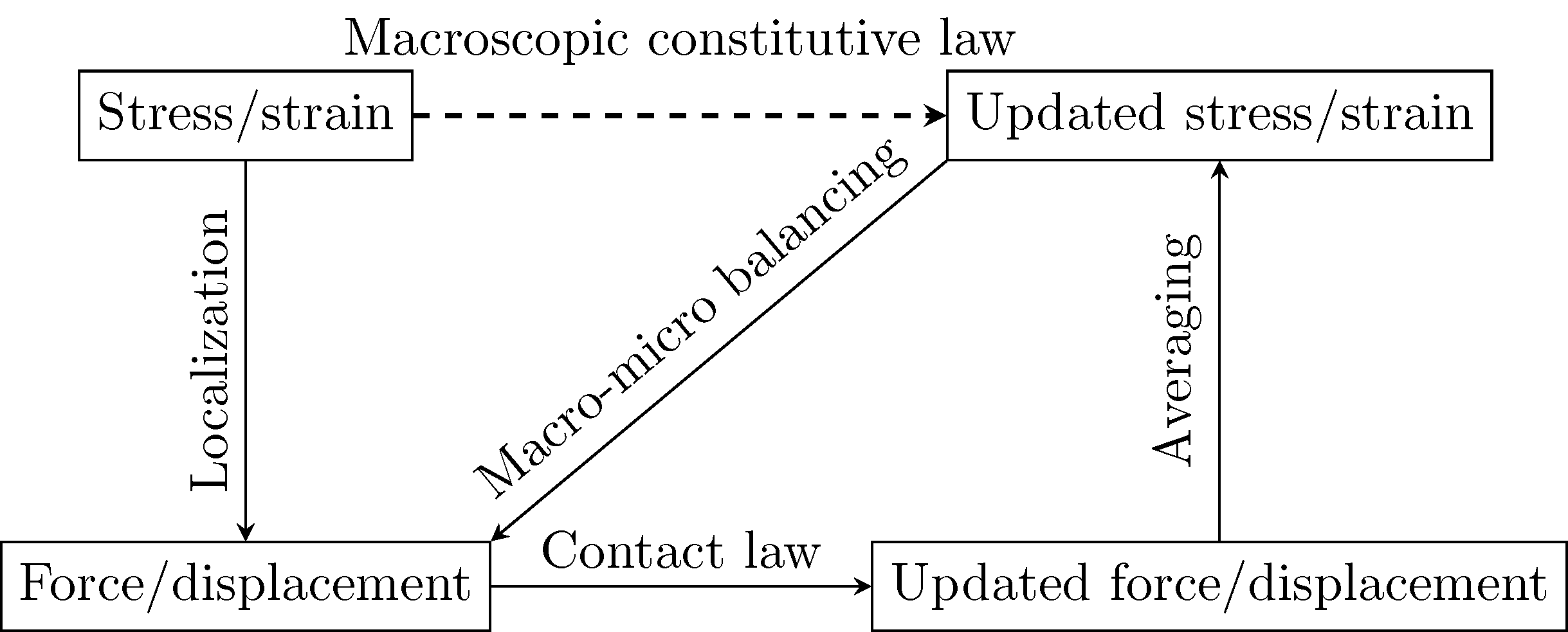
Figure 1: Basic micromechanical framework
Kinematic 假设
Kinematic 假设 下的应力应变关系: \[
\mathrm{d}\boldsymbol{\sigma}_{ij}=\mathbf{C}_{ijkl}\mathrm{d}\boldsymbol{\varepsilon}_{kl},\mathbf{C}_{ijkl}=\dfrac{1}{V}\sum_{c=1}^N{\mathbf{k}_{jl}^c \mathbf{l}_i^c \mathbf{l}_k^c}
\tag{1}\] Voigt 表示法下的刚度矩阵: \[
% \mathbf{C}_{ij}=\begin{bmatrix}
% \lambda+2\mu+c_1F_{11} & \lambda F_{33}^{[-2/7]} & \lambda F_{22}^{[-2/7]} & c_3F_{23} & c_3F_{13} & \dfrac{2}{7}\lambda F_{12} \\
% & \lambda+2\mu+c_1F_{22} & \lambda F_{11}^{[-2/7]} & \dfrac{6}{7}\lambda F_{23} & \dfrac{2}{7}\lambda F_{13} & c_3F_{12} \\
% & & \lambda+2\mu+c_1F_{33} & \dfrac{2}{7}\lambda F_{23} & \dfrac{6}{7}\lambda F_{13} & \dfrac{6}{7}\lambda F_{12} \\
% & & & \mu-c_2F_{11} & c_2F_{12} & c_2F_{13} \\
% & & & & \mu-c_2F_{22} & c_2F_{23} \\
% \text{Sym.} & & & & & \mu-c_2F_{33}
% \end{bmatrix}
\begin{aligned}
&\mathbf{C}_{ij}=\begin{bmatrix}
\mathbf{C}_1 & \mathbf{C}_3 \\
\mathbf{C}_3^{\mathsf{T}} & \mathbf{C}_2
\end{bmatrix} \\
&\mathbf{C}_1=\begin{bmatrix}
\lambda+2\mu+c_1F_{11} & \lambda F_{33}^{[-2/7]} & \lambda F_{22}^{[-2/7]} \\
& \lambda+2\mu+c_1F_{22} & \lambda F_{11}^{[-2/7]} \\
\text{Sym.} & & \lambda+2\mu+c_1F_{33}
\end{bmatrix} \\
&\mathbf{C}_2=\begin{bmatrix}
\mu-c_2F_{11} & c_2F_{12} & c_2F_{13} \\
& \mu-c_2F_{22} & c_2F_{23} \\
\text{Sym.} & & \mu-c_2F_{33}
\end{bmatrix} \\
&\mathbf{C}_3=\begin{bmatrix}
c_3F_{23} & c_3F_{13} & \dfrac{2}{7}\lambda F_{12} \\
\dfrac{6}{7}\lambda F_{23} & \dfrac{2}{7}\lambda F_{13} & c_3F_{12} \\
\dfrac{2}{7}\lambda F_{23} & \dfrac{6}{7}\lambda F_{13} & \dfrac{6}{7}\lambda F_{12} \\
\end{bmatrix}
\end{aligned}
\tag{2}\] 式中 \(F_{ij}^{[x]}=1+xF_{ij}\),其它常数为: \[
\begin{aligned}
&v=\dfrac{3V}{2Nr^3}, E=\dfrac{2k_n}{rv}\dfrac{2+3\alpha}{4+\alpha}, \nu=\dfrac{1-\alpha}{4+\alpha} \\
&\lambda=\dfrac{E\nu}{\left(1+\nu\right)\left(1-2\nu\right)}, \mu=G=\dfrac{E}{2\left(1+\nu\right)} \\
&c_1=\dfrac{4\left(8\lambda+7\mu\right)}{35}, c_2=\dfrac{3\lambda+7\mu}{35}, c_3=\dfrac{2\left(\lambda+14\mu\right)}{35}
\end{aligned}
\tag{3}\]
Static 假设
Static 假设 下的应力应变关系: \[
\mathrm{d}\boldsymbol{\varepsilon}_{ij}\!=\!\mathbf{S}_{ijkl}\mathrm{d}\boldsymbol{\sigma}_{kl},\mathbf{S}_{ijkl}\!=\!\dfrac{1}{V}\sum_{c=1}^N{\left(\mathbf{k}_{jl}^c\right)^{-1} \mathbf{l}_m^c \mathbf{l}_n^c \mathbf{A}_{mi} \mathbf{A}_{nk}}
\tag{4}\] Voigt 表示法下的柔度矩阵: \[
% \mathbf{S}_{ij}^\prime=\begin{bmatrix}
% \dfrac{F_{11}^{[c_4]}}{E} & -\dfrac{\nu}{E}F_{33}^{[-2/7]} & -\dfrac{\nu}{E}F_{22}^{[-2/7]} & \dfrac{c_6F_{23}}{E} & \dfrac{c_6F_{13}}{E} & -\dfrac{\nu}{E}\dfrac{2}{7}F_{12} \\
% & \dfrac{F_{22}^{[c_4]}}{E} & -\dfrac{\nu}{E}F_{11}^{[-2/7]} & -\dfrac{\nu}{E}\dfrac{6}{7}F_{23} & -\dfrac{\nu}{E}\dfrac{2}{7}F_{13} & \dfrac{c_6F_{12}}{E} \\
% & & \dfrac{F_{33}^{[c_4]}}{E} & -\dfrac{\nu}{E}\dfrac{2}{7}F_{23} & -\dfrac{\nu}{E}\dfrac{6}{7}F_{13} & -\dfrac{\nu}{E}\dfrac{6}{7}F_{12} \\
% & & & \dfrac{1}{G}F_{11}^{[-1/5]} & \dfrac{c_5F_{12}}{E} & \dfrac{c_5F_{13}}{E} \\
% & & & & \dfrac{1}{G}F_{22}^{[-1/5]} & \dfrac{c_5F_{23}}{E} \\
% \text{Sym.} & & & & & \dfrac{1}{G}F_{33}^{[-1/5]} \\
% \end{bmatrix}
\begin{aligned}
&\mathbf{S}_{ij}^\prime=\begin{bmatrix}
\mathbf{S}_1 & \mathbf{S}_3 \\
\mathbf{S}_3^{\mathsf{T}} & \mathbf{S}_2
\end{bmatrix} \\
&\mathbf{S}_1=\begin{bmatrix}
\dfrac{1}{E}F_{11}^{[c_4]} & -\dfrac{\nu}{E}F_{33}^{[-2/7]} & -\dfrac{\nu}{E}F_{22}^{[-2/7]} \\
& \dfrac{1}{E}F_{22}^{[c_4]} & -\dfrac{\nu}{E}F_{11}^{[-2/7]} \\
\text{Sym.} & & \dfrac{1}{E}F_{33}^{[c_4]}
\end{bmatrix} \\
&\mathbf{S}_2=\begin{bmatrix}
\dfrac{1}{G}F_{11}^{[-1/5]} & \dfrac{c_5F_{12}}{E} & \dfrac{c_5F_{13}}{E} \\
& \dfrac{1}{G}F_{22}^{[-1/5]} & \dfrac{c_5F_{23}}{E} \\
\text{Sym.} & & \dfrac{1}{G}F_{33}^{[-1/5]}
\end{bmatrix} \\
&\mathbf{S}_3=\begin{bmatrix}
\dfrac{c_6F_{23}}{E} & \dfrac{c_6F_{13}}{E} & -\dfrac{\nu}{E}\dfrac{2}{7}F_{12} \\
-\dfrac{\nu}{E}\dfrac{6}{7}F_{23} & -\dfrac{\nu}{E}\dfrac{2}{7}F_{13} & \dfrac{c_6F_{12}}{E} \\
-\dfrac{\nu}{E}\dfrac{2}{7}F_{23} & -\dfrac{\nu}{E}\dfrac{6}{7}F_{13} & -\dfrac{\nu}{E}\dfrac{6}{7}F_{12} \\
\end{bmatrix}
\end{aligned}
\tag{5}\] 式中的常数为: \[
\begin{aligned}
&E=\dfrac{2k_n}{rv}\dfrac{5\alpha}{2+3\alpha}, \nu=\dfrac{1-\alpha}{2+3\alpha}, G=\dfrac{E}{2\left(1+\nu\right)} \\
&c_4=\dfrac{2\left(7-9\nu\right)}{35}, c_5=\dfrac{2\left(7+\nu\right)}{35}, c_6=\dfrac{2\left(7+6\nu\right)}{35}
\end{aligned}
\tag{6}\]
解析解的验证
![]()
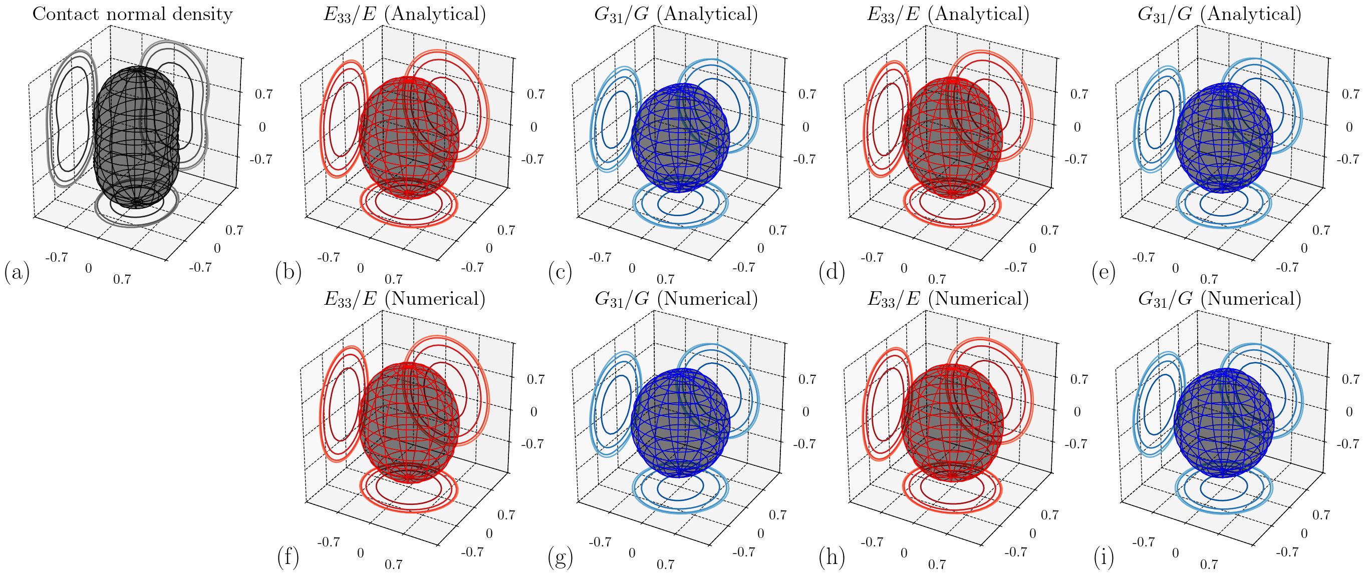
Figure 2: Comparison between analytical and numerical solutions of \(E_{33}/E\) and \(G_{31}/G\) for static and kinematic hypotheses: (a) contact normal density; (b)(c)(f)(g) analytical and numerical solutions of \(E_{33}/E\) and \(G_{31}/G\) for static hypothesis; (d)(e)(h)(i) analytical and numerical solutions for kinematic hypothesis
各向同性时两种假设的应力应变关系
![]()
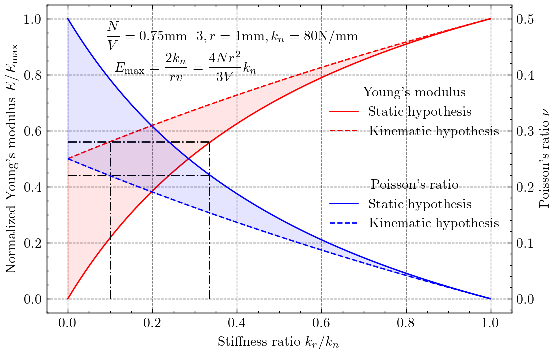
Figure 3: Young’s modulus and Poisson’s ratio for static and kinematic hypotheses under isotropic stress conditions
横观各向同性时两种假设的应力应变关系
![]()
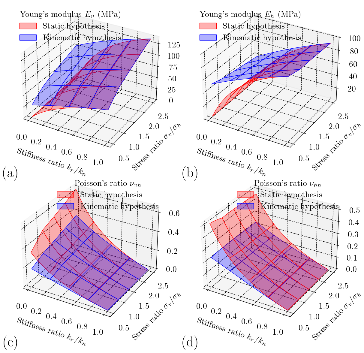
Figure 4: Young’s modulus and Poisson’s ratio for static and kinematic hypotheses under anisotropic stress conditions: (a) \(E_v\); (b) \(E_h\); (c) \(\nu_{vh}\); (d) \(\nu_{hh}\)
各向同性加载
![]()
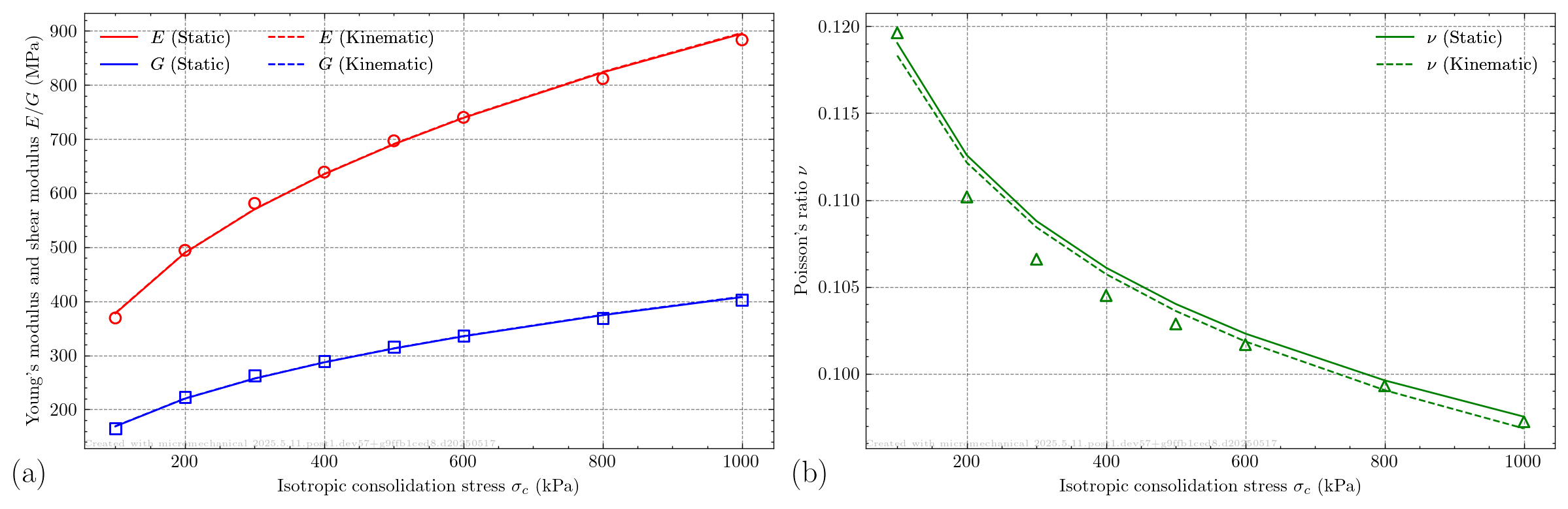
Figure 5: Young’s modulus, shear modulus and Poisson’s ratio at isotropic stress states: (a) Young’s modulus; (b) Poisson’s ratio
各向异性加载
![]()
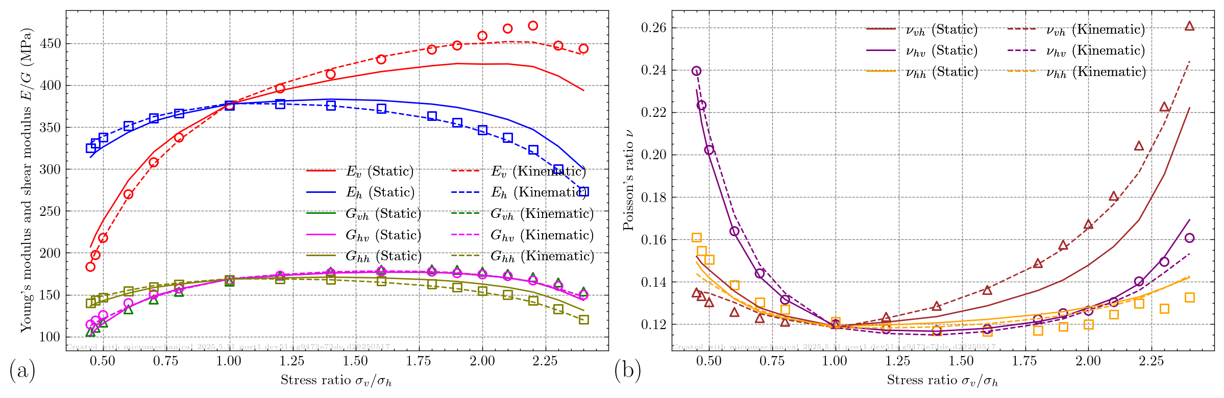
Figure 6: Young’s modulus, shear modulus and Poisson’s ratio at anisotropic stress states: (a) Young’s modulus and shear modulus; (b) Poisson’s ratio
应力、组构以及模量各向异性之间的关系
![]()
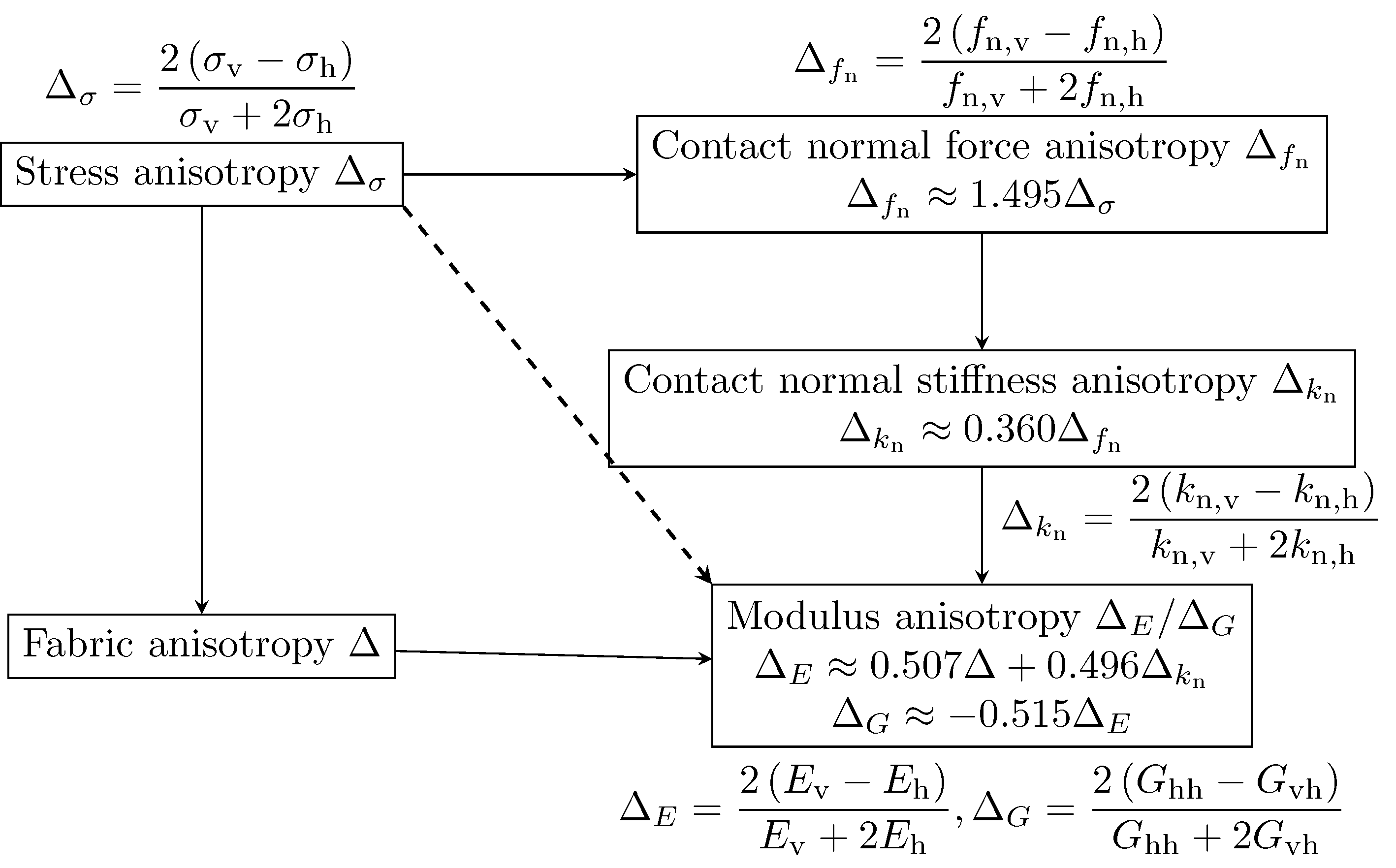
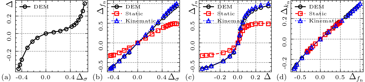
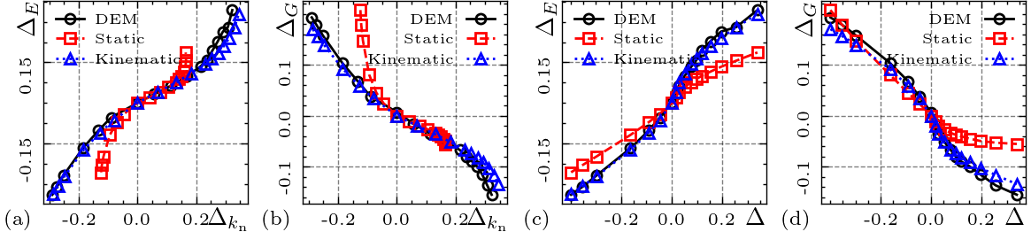
Figure 7: Relationships between fabric, stress, contact normal force, contact normal stiffness, Young’s modulus and shear modulus anisotropies
应力各向异性对接触法向力和接触法向刚度各向异性的影响
![]()
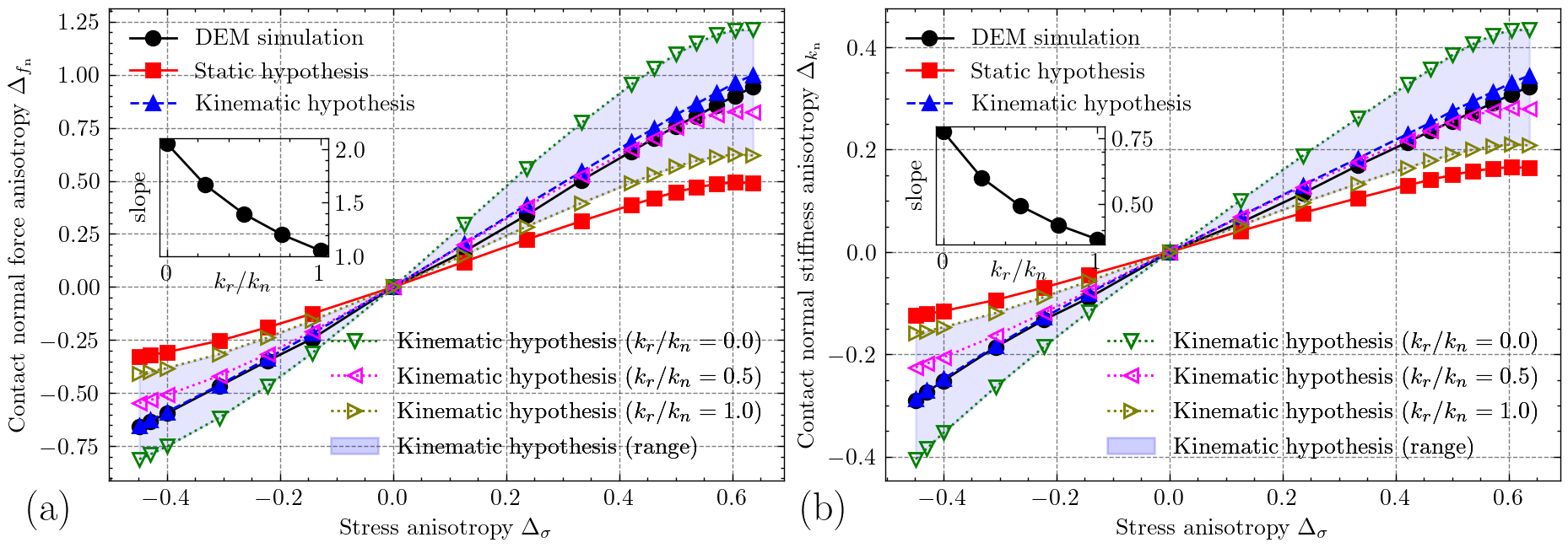
Figure 10: Effects of stress anisotropy on contact normal force and contact normal stiffness anisotropies: (a) contact normal force anisotropy; (b) contact normal stiffness anisotropy
不同各向异性之间的线性关系
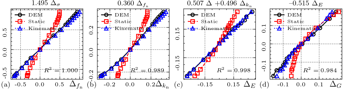
![Regressions between anisotropies: (a) stress anisotropy vs. contact normal force anisotropy; (b) contact normal force anisotropy vs. contact normal stiffness anisotropy; (c) fabric and contact normal stiffness anisotropies vs. Young’s modulus anisotropy; (d) Young’s modulus anisotropy vs. shear modulus anisotropy]() \[
\begin{aligned}
&\Delta_E \approx \dfrac{1}{2}\Delta+\dfrac{c}{4}\Delta_{\sigma}, c \ge \dfrac{2}{3} \\
&\Delta_G \approx -\left(\dfrac{1}{4}\Delta+\dfrac{c}{8}\Delta_{\sigma}\right)
\end{aligned}
\tag{7}\] \[
\begin{aligned}
\dfrac{E_v}{E_h} &\approx \dfrac{2\left(2+\Delta\right)\left(\mathrm{SR}+2\right)+2c\left(\mathrm{SR}-1\right)}{\left(4-\Delta\right)\left(\mathrm{SR}+2\right)-c\left(\mathrm{SR}-1\right)} \\
\dfrac{G_{vh}}{G_{hh}} &\approx \dfrac{2\left(4+\Delta\right)\left(\mathrm{SR}+2\right)+2c\left(\mathrm{SR}-1\right)}{\left(8-\Delta\right)\left(\mathrm{SR}+2\right)-c\left(\mathrm{SR}-1\right)}
\end{aligned}
\tag{8}\]
\[
\begin{aligned}
&\Delta_E \approx \dfrac{1}{2}\Delta+\dfrac{c}{4}\Delta_{\sigma}, c \ge \dfrac{2}{3} \\
&\Delta_G \approx -\left(\dfrac{1}{4}\Delta+\dfrac{c}{8}\Delta_{\sigma}\right)
\end{aligned}
\tag{7}\] \[
\begin{aligned}
\dfrac{E_v}{E_h} &\approx \dfrac{2\left(2+\Delta\right)\left(\mathrm{SR}+2\right)+2c\left(\mathrm{SR}-1\right)}{\left(4-\Delta\right)\left(\mathrm{SR}+2\right)-c\left(\mathrm{SR}-1\right)} \\
\dfrac{G_{vh}}{G_{hh}} &\approx \dfrac{2\left(4+\Delta\right)\left(\mathrm{SR}+2\right)+2c\left(\mathrm{SR}-1\right)}{\left(8-\Delta\right)\left(\mathrm{SR}+2\right)-c\left(\mathrm{SR}-1\right)}
\end{aligned}
\tag{8}\]
应力、组构以及模量各向异性之间的关系
![]()
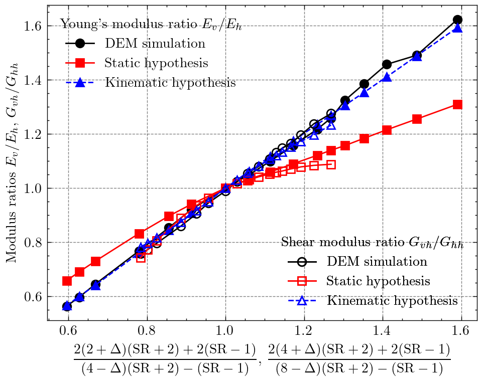
Figure 11: Comparison between Young’s modulus and shear modulus ratios from DEM simulations and predictions
本学期工作总结及接下来的工作计划
- 工作总结
- 撰写了基于 SANISAND 模型的各向异性微观接触模型的中英文文章
- 推导两种均质化假设的小应变刚度,并使用 DEM 模拟数据验证了小应变刚度
- 撰写了小应变刚度模拟的英文文章
- 工作计划
- 将多尺度微观力学模型写成 ABAQUS UMAT 子程序
- 使用微观力学模型模拟不同基础尺寸、不同各向异性程度、不同沉积角及不同孔隙比的基础极限承载力
 \[
\begin{aligned}
&\Delta_E \approx \dfrac{1}{2}\Delta+\dfrac{c}{4}\Delta_{\sigma}, c \ge \dfrac{2}{3} \\
&\Delta_G \approx -\left(\dfrac{1}{4}\Delta+\dfrac{c}{8}\Delta_{\sigma}\right)
\end{aligned}
\tag{7}\] \[
\begin{aligned}
\dfrac{E_v}{E_h} &\approx \dfrac{2\left(2+\Delta\right)\left(\mathrm{SR}+2\right)+2c\left(\mathrm{SR}-1\right)}{\left(4-\Delta\right)\left(\mathrm{SR}+2\right)-c\left(\mathrm{SR}-1\right)} \\
\dfrac{G_{vh}}{G_{hh}} &\approx \dfrac{2\left(4+\Delta\right)\left(\mathrm{SR}+2\right)+2c\left(\mathrm{SR}-1\right)}{\left(8-\Delta\right)\left(\mathrm{SR}+2\right)-c\left(\mathrm{SR}-1\right)}
\end{aligned}
\tag{8}\]
\[
\begin{aligned}
&\Delta_E \approx \dfrac{1}{2}\Delta+\dfrac{c}{4}\Delta_{\sigma}, c \ge \dfrac{2}{3} \\
&\Delta_G \approx -\left(\dfrac{1}{4}\Delta+\dfrac{c}{8}\Delta_{\sigma}\right)
\end{aligned}
\tag{7}\] \[
\begin{aligned}
\dfrac{E_v}{E_h} &\approx \dfrac{2\left(2+\Delta\right)\left(\mathrm{SR}+2\right)+2c\left(\mathrm{SR}-1\right)}{\left(4-\Delta\right)\left(\mathrm{SR}+2\right)-c\left(\mathrm{SR}-1\right)} \\
\dfrac{G_{vh}}{G_{hh}} &\approx \dfrac{2\left(4+\Delta\right)\left(\mathrm{SR}+2\right)+2c\left(\mathrm{SR}-1\right)}{\left(8-\Delta\right)\left(\mathrm{SR}+2\right)-c\left(\mathrm{SR}-1\right)}
\end{aligned}
\tag{8}\]